Some time ago I published a blog post with the title Know your data structures!. In this previous post I explained how I improved the running time of a genetic algorithm. I promised to go more into detail about other noteworthy things in the code in a separate article since not everything was straightforward when porting the genetic algorithms code from python to R.
Contents
The Learning Club activity
The current Learning Club activity is about Genetic Algorithms. I have had a heuristics class at university and was always quite interested in the topic. So after skipping a few activities in the learning club I finally managed to implement something again.
Check out the activity description: Genetic Algorithms Map Path – Activity Description & Resources | www.becomingadatascientist.com forum
Original code
My implementation is based on code by Randy Olson. Here you can find his jupyter notebook.
My code
My code can be found in my git repository
16-genetic-algorithms.
Details of the code
The code mainly consists of four files:
- data_store_helper.R
- genetic_algorithm.R
- list_helper.R
- run_algorithm.R
There is also the file timing_distance_functions.R which I used for the analysis in this blog post about the code speedup.
The file genetic_algorithm.R contains the algorithm and will be explained further.
Entry point run_genetic_algorithm
The entry point of the program is the function run_genetic_algorithm, which takes a distance_matrix, a list all_waypoints and the parameters generations and population_size.
After some initialisations, the program repeatedly takes the 10% fittest candidates and fills a new population with them.
The population fitness is computed according to a fitness function (in this case simply the distance between two waypoints):
    population_fitness <- list()
    for (i in 1:length(population)) {
      if (!contains(population_fitness, population[[i]])) {
        fit <- compute_fitness_fast(distance_matrix, population[[i]])
        agent_fitness <- list("agent"=population[[i]], "fitness"=unname(fit))
        population_fitness[[length(population_fitness)+1]] <- agent_fitness
      }
    }
The interesting part is how the next population is determined. For each of the top 10% candidates from the current population, 10 offspring are generated for the next generations population.
- 1 is copied to the next population without modifications
- 2 are generated by introducing point mutations into the candidate
- 7 are generated by a shuffle mutation applied to the candidate
mutate_agent
The function mutate_agent is used to take an agent and introduce some mutations into it. For the travelling salesman problem this means to take 2 waypoints at random and swapping their position in the path.
parameter max_mutations: In the current implementation, also a number max_mutations can be passed to the function. From my understanding of the code this is not really a maximum but the exact number of mutations that are introduced.
Improving swapping: In the original code there was a while loop that selected swap_index2 until it was different from swap_index1. In my code I used the line swap_index2 <- sample((1:length(agent_genome))[-swap_index1], 1) to pick one index from all possible indices except for the already picked one (-swap_index1).
mutate_agent <- function(agent_genome, max_mutations=3) {
  num_mutations <- sample(1:max_mutations, 1)
  for (mutation in 1:num_mutations) {
    swap_index1 <- sample(1:length(agent_genome), 1)

    swap_index2 <- sample((1:length(agent_genome))[-swap_index1], 1)

    temp_agent_genome <- agent_genome[swap_index1]
    agent_genome[swap_index1] <- agent_genome[swap_index2]
    agent_genome[swap_index2] <- temp_agent_genome
  }

  return (agent_genome)
}
shuffle_mutation
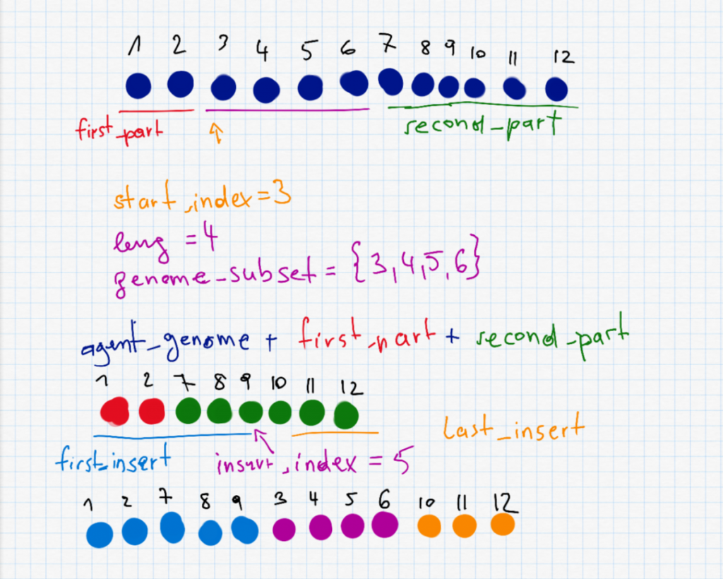
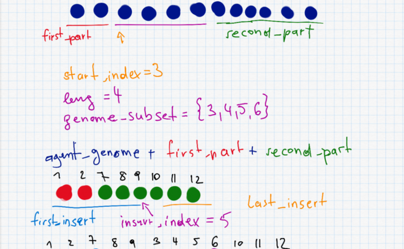
This is probably the most interesting part and also the most complex one. To do a shuffle, we need to randomly selected a start_index and a length leng to decide which part (waypoints) of the route to shuffle. The two parts before and after (first_part and second_part) are put together as the new agent_genome. Furthermore we have to randomly select the insert_index which is somewhere on the new (shorter) agent. The shuffle is described in the following picture.

second_part" I accidentally wrote a + instead of =.
shuffle_mutation <- function(agent_genome) {

  start_index <- sample(1:length(agent_genome), 1)
  leng <- sample(1:min(length(agent_genome)-start_index + 1,20), 1)

  genome_subset <- agent_genome[start_index:(start_index + leng - 1)]
  first_part <- 0:(start_index-1)
  second_part <- c()
  if (start_index + leng <= length(agent_genome)) {
    second_part <- (start_index + leng):length(agent_genome)
  }
  agent_genome <- c(agent_genome[first_part], agent_genome[second_part])

  insert_index <- sample(0:(length(agent_genome)), 1)
  first_insert <- 0:insert_index
  last_insert <- c()
  if (insert_index < length(agent_genome)) {
    last_insert <- (insert_index+1):length(agent_genome)
  }
  agent_genome <- c(agent_genome[first_insert], genome_subset, agent_genome[last_insert])
  agent_genome <- agent_genome[!is.na(agent_genome)]

  return(agent_genome)
}
Why are there 0's although R counts from 1? I found this neat property of R when debugging my code. If I start my sequence with 0 it behaves different than when I start it with 1. If I write 0:insert_index and insert_index is 0 (which means the sequence is inserted before the very first element), the sequence is empty and it is ignored when I use it for indexing. If I write 1:insert_index and insert_index is 0, the result is an array 1 0 and I access the first element although I don't want to (see agent_genome[first_insert]).
What's with the two if conditions? I'm pretty sure this is not the best way to do it. But it helps with the cases that (1) the shuffled part includes the last element and (2) that the insertion should take place at the very end of the sequence.
Why do you check for NA in the last line before the return? I'm also sure that this is not the nicest way to do it, but in the case that I access something that's not there, I end up with NA's at the beginning or end of my new genome.
Now it's your turn
Give me feedback or do the activity in the learning club yourself!

