Just a few days ago I stated the following on Twitter:

Just reduced the runtime of an algorithm from 9 hours to 3 min. by using a different data structure… Know you data structures 🙂 #rstats

— Verena Haunschmid (@ExpectAPatronum) May 1, 2017

Since my tweet has been liked and shared a lot, I thought I’d backup my claim with a small experiment.

I’ve used my 6 year old Macbook Pro, so if you try this on your computer everything is probably faster!

Background

The problem I tried to solve was to implement a genetic algorithm initially programmed in python by Randy Olson. I’m participating in a Data Science Learning Club and the current activity was about Genetic Algorithms. The jupyter notebook by Randy was given as an example and we can always choose by ourselves how we want to approach a topic in the learning club. Since I’m currently not doing much in R, I decided it would be a good practice to stay up-to-date.

Here is the complete code for the assignment in my git repo.

Porting the code

There will be a lot more detail about the genetic algorithm code in a future blog post. Basically porting it was straight forward. I had to take care of the indices (R starts counting at 1, python at 0) and for me, Python’s indexing is not very intuitive. But I managed to create a running program. Randy’s settings were to use 5000 generations and 100 populations. His python code only took a couple of minutes on my computer.

Running time

When I first wanted to run my R code I immediately noticed something was wrong. It needed approximately 7 seconds for one generation, which would result in a complete running time of 9 hours! I stopped the program and tried to investigate what was going on.

I debugged the code and found which part of the function run_genetic_algorithm was the slowest:

  for (generation in 1:generations) {
    population_fitness <- list()
    for (i in 1:length(population)) {
      if (!contains(population_fitness, population[[i]])) {
        fit <- compute_fitness_fast(distance_matrix, population[[i]]) # here I had used the method compute_fitness instead of compute_fitness_fast
        agent_fitness <- list("agent"=population[[i]], "fitness"=unname(fit))
        population_fitness[[length(population_fitness)+1]] <- agent_fitness
      }
    }

This part accounted for more than 5 seconds of the 7 seconds per loop!

At first I thought the loop was the problem because as we all know you should avoid loops in R and use apply, lapply and so on ...

So as a first step I changed the implementation of compute_fitness.

This is the old implementation:

compute_fitness <- function(data_store, solution) {
  solution_fitness <- 0.0
  for (index in 2:length(solution)) {
    waypoint1 <- solution[index - 1]
    waypoint2 <- solution[index]
    solution_fitness <- solution_fitness + waypoint_distances(data_store, waypoint1, waypoint2)
  }
  return(solution_fitness)
}

This was the first improvement using lapply:

compute_fitness_fast <- function(distance_matrix, solution) {
  fitness_list <- lapply(2:length(solution), function(index) {
    waypoint1 <- solution[index - 1]
    waypoint2 <- solution[index]
    waypoint_distances(data_store, waypoint1, waypoint2)
  })
  return(Reduce("+", fitness_list))
}

This made it slightly better but only cut about half a second from the 5 seconds. Overall this would not reduce the running time by very much. Also notice the use of the method Reduce. While researching on how to improve my code, I also found out about Common Higher-Order Functions in Functional Programming Languages, which I didn't know existed in R (you might have heard about map/reduce operations before). That's very practical!

Don't always use data.frames

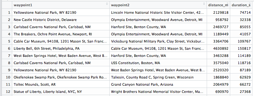
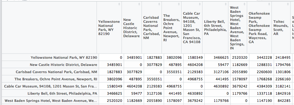
Luckily I had the idea that maybe the data.frame where I stored the distances was the problem, since I had to do thousands of lookups. I researched a little and found out that matrices have better memory performance. Also the typical structure for storing pairwise distances is a distance matrix... I'm not sure if that's the whole story and what else is going on when I lookup something in a data.frame, but I thought it's worth a try.
I wrote a small script to transform the data.frame into a matrix:

build_distance_matrix <- function(data_store) {
  all_waypoints <- union(data_store$waypoint1, data_store$waypoint2)
  n <- length(all_waypoints)
  dist_m <- matrix(rep(0, n*n), nrow=n)
  for (i in 1:n) {
    for (j in 1:n) {
      if (i == j) {
        dist_m[i, j] <- 0
      } else if (i < j) {
        dist_ij <- unlist(waypoint_distances(data_store, all_waypoints[i], all_waypoints[j]))
        dist_m[i, j] <- dist_ij
        dist_m[j, i] <- dist_ij
      }
    }
  }
  colnames(dist_m) <- rownames(dist_m) <- all_waypoints
  return(dist_m)
}

Since I use the city names as column and row names, I can directly use them to access the distance!

And I changed the method compute_fitness_fast to this:

compute_fitness_fast <- function(distance_matrix, solution) {
  fitness_list <- lapply(2:length(solution), function(index) {
    waypoint1 <- solution[index - 1]
    waypoint2 <- solution[index]
    distance_matrix[waypoint1, waypoint2]
  })
  return(Reduce("+", fitness_list))
}

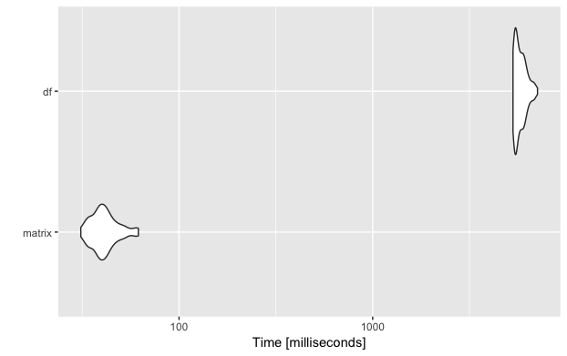
And yay, I immediately noticed a huge speedup from 5.619 seconds to 0.042 seconds per generation, which is 133 times faster!

microbenchmark

To do the comparison properly, I used the R package microbenchmark (link to documentation). You can pass one or more functions/expressions to the microbenchmark method and tell it how often to run the functions for the comparison.

res <- microbenchmark(matrix=({
  population_fitness <- list()
  for (agent_genome in population) {
    if (!contains(population_fitness, agent_genome)) {
      fit <- compute_fitness_fast(dist_matrix, agent_genome)
      agent_fitness <- list("agent"=agent_genome, "fitness"=unname(fit))
      population_fitness[[length(population_fitness)+1]] <- agent_fitness
    }
  }}),
  df=({
    population_fitness <- list()
    for (agent_genome in population) {
      if (!contains(population_fitness, agent_genome)) {
        fit <- compute_fitness(data_store_us, agent_genome)
        agent_fitness <- list("agent"=agent_genome, "fitness"=unname(fit))
        population_fitness[[length(population_fitness)+1]] <- agent_fitness
      }
    }}),
  times = 100)

If you want to plot the results using autoplot it is important to give the functions names (e.g. matrix and df) otherwise it will try to put the whole expressions onto the y axis labels.

And as you can see, just by replacing the data.frame by the more suitable matrix, this important part of my algorithm became a lot faster!

>> Using the microbenchmark package to compare the execution time of R expressions | gettinggeneticsdone.com

Takeaway from this post

What I learned from this problem and maybe also you, is that you should never just use the data structure that is given. I simply read the csv file that was stored by the Jupyter notebook (it seems to be very efficient in Python) and used the first data structure that seemed to fit. In this case it would have made sense to think about what the underlying structure of the data is. There is one number for each pair of cities, which makes a matrix a real good fit. The name distance matrix already suggests how it should be stored 🙂

I'd also like to know more about the underlying reason why there is such a huge distance. If you have any more resources, I'd like to read/hear about it!